Pure Data and libpd: Integrating with Native Code for Interactive Testing

Over the past couple of years, I’ve built up a nice library of DSP code, including effects, oscillators, and utilities. One thing that always bothered me however, is how to test this code in an efficient and reliable way. The two main methods I have used in the past have their pros and cons, but ultimately didn’t satisfy me.

One is to process an effect or generate a source into a wave file that I can open with an audio editor so I can listen to the result and examine the output. This method is okay, but it is tedious and doesn’t allow for real-time adjustment of parameters or any sort of instant feedback.

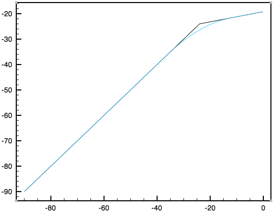
For effects like filters, I can also generate a text file containing the frequency/phase response data that I can view in a plotting application. This is useful in some ways, but this is audio — I want to hear it!

Lately I’ve gotten to know Pure Data a little more, so I thought about using it for interactive testing of my DSP modules. On its own, Pure Data does not interact with code of course, but that’s where libpd comes in. This is a great library that wraps up much of Pure Data’s functionality so that you can use it right from your own code (it works with C, C++, Objective-C, Java, and others). Here is how I integrated it with my own code to set up a nice flexible testing framework; and this is just one application of using libpd and Pure Data together — the possiblities go far beyond this!

First we start with the Pure Data patches. The receiver patch is opened and maintained in code by libpd, and has two responsiblities: 1) generate a test tone that the effect is applied to, and 2) receive messages from the control patch and dispatch them to C++.

Receiver patch, opened by libpd.

The control patch is opened in Pure Data and acts as the interactive patch. It has controls for setting the frequency and volume of the synthesizer tone that acts as the source, as well as controls for the filter effect that is being tested.

Control patch, opened in Pure Data, and serves as the interactive UI for testing.

As can be seen from the patches above, they communicate to each other via the netsend/netreceive objects by opening a port on the local machine. Since I’m only sending simple data to the receiver patch, I opted to use UDP over TCP as the network protocol. (Disclaimer: my knowledge of network programming is akin to asking “what is a for loop”).

Hopefully the purpose of these two patches is clear, so we can now move on to seeing how libpd brings it all together in code. It is worth noting that libpd does not output audio to the hardware, it only processes the data. Pure Data, for example, commonly uses Portaudio to send the audio data to the sound card, but I will be using Core Audio instead. Additionally, I’m using the C++ wrapper from libpd.

An instance of PdBase is first created with the desired intput/output channels and sample rate, and a struct contains data that will need to be held on to that will become clear further on.

struct TestData
{
    AudioUnit outputUnit;
    EffectProc effectProc;

    PdBase* pd;
    Patch pdPatch;
    float* pdBuffer;
    int pdTicks;
    int pdSamplesPerBlock;

    CFRingBuffer<float> ringBuffer;
    int maxFramesPerSlice;
    int framesInReserve;
};

int main(int argc, const char * argv[])
{
    PdBase pd;
    pd.init(0, 2, 48000); // No input needed for tests.

    TestData testData;
    testData.pd = &pd;
    testData.pdPatch = pd.openPatch("receiver.pd", ".");
}

Next, we ask Core Audio for an output Audio Unit that we can use to send audio data to the sound card.

int main(int argc, const char * argv[])
{
    PdBase pd;
    pd.init(0, 2, 48000); // No input needed for tests.

    TestData testData;
    testData.pd = &pd;
    testData.pdPatch = pd.openPatch("receiver.pd", ".");

    {
        AudioComponentDescription outputcd = {0};
        outputcd.componentType = kAudioUnitType_Output;
        outputcd.componentSubType = kAudioUnitSubType_DefaultOutput;
        outputcd.componentManufacturer = kAudioUnitManufacturer_Apple;

        AudioComponent comp = AudioComponentFindNext(NULL, &outputcd);
        if (comp == NULL)
        {
            std::cerr << "Failed to find matching Audio Unit.\n";
            exit(EXIT_FAILURE);
        }

        OSStatus error;
        error = AudioComponentInstanceNew(comp, &testData.outputUnit);
        if (error != noErr)
        {
            std::cerr << "Failed to open component for Audio Unit.\n";
            exit(EXIT_FAILURE);
        }

        Float64 sampleRate = 48000;
        UInt32 dataSize = sizeof(sampleRate);
        error = AudioUnitSetProperty(audioUnit,
                                     kAudioUnitProperty_SampleRate,
                                     kAudioUnitScope_Input,
                                     0, &sampleRate, dataSize);

        AudioUnitInitialize(audioUnit);
    }
}

The next part needs some explanation, because we need to consider how the Pure Data patch interacts with Core Audio’s render callback function that we will provide. This function will be called continuously on a high priority thread with a certain number of frames that we need to fill with audio data. Pure Data, by default, processes 64 samples per channel per block. It’s unlikely that these two numbers (the number of frames that Core Audio wants and the number of frames processed by Pure Data) will always agree. For example, in my initial tests, Core Audio specified its maximum block size to be 512 frames, but it actually asked for 470 & 471 (alternating) when it ran. Rather than trying to force the two to match block sizes, I use a ring buffer as a medium between the two — that is, read sample data from the opened Pure Data patch into the ring buffer, and then read from the ring buffer into the buffers provided by Core Audio.

Fortunately, Core Audio can be queried for the maximum number of frames it will ask for, so this will determine the number of samples we read from the Pure Data patch. We can read a multiple of Pure Data’s 64-sample block by specifying a value for “ticks” in libpd, and this value will just be equal to the maximum frames from Core Audio divided by Pure Data’s block size. The actual number of samples read/processed will of course be multiplied by the number of channels (2 in this case for stereo).

The final point on this is to handle the case where the actual number of frames processed in a block is less than the maximum. Obviously it would only take a few blocks for the ring buffer’s write pointer to catch up with the read pointer and cause horrible audio artifacts. To account for this, I make the ring buffer twice as long as the number of samples required per block to give it some breathing room, and also keep track of the number of frames in reserve currently in the ring buffer at the end of each block. When this number exceeds the number of frames being processed in a block, no processing from the patch occurs, giving the ring buffer a chance to empty out its backlog of frames.

int main(int argc, const char * argv[])
{
    <snip> // As above.

    UInt32 framesPerSlice;
    UInt32 dataSize = sizeof(framesPerSlice);
    AudioUnitGetProperty(testData.outputUnit,
                         kAudioUnitProperty_MaximumFramesPerSlice,
                         kAudioUnitScope_Global,
                         0, &framesPerSlice, &dataSize);
    testData.pdTicks = framesPerSlice / pd.blockSize();
    testData.pdSamplesPerBlock = (pd.blockSize() * 2) * testData.pdTicks; // 2 channels for stereo output.
    testData.maxFramesPerSlice = framesPerSlice;

    AURenderCallbackStruct renderCallback;
    renderCallback.inputProc = AudioRenderProc;
    renderCallback.inputProcRefCon = &testData;
    AudioUnitSetProperty(testData.outputUnit,
                         kAudioUnitProperty_SetRenderCallback,
                         kAudioUnitScope_Input,
                         0, &renderCallback, sizeof(renderCallback));

    testData.pdBuffer = new float[testData.pdSamplesPerBlock];
    testData.ringBuffer.resize(testData.pdSamplesPerBlock * 2); // Twice as long as needed in order to give it some buffer room.
    testData.effectProc = EffectProcess;
}

With the output Audio Unit and Core Audio now set up, let’s look at the render callback function. It reads the audio data from the Pure Data patch if needed into the ring buffer, which in turn fills the buffer list provided by Core Audio. The buffer list is then passed on to the callback that processes the effect being tested.

OSStatus AudioRenderProc (void *inRefCon,
                          AudioUnitRenderActionFlags *ioActionFlags,
                          const AudioTimeStamp *inTimeStamp,
                          UInt32 inBusNumber,
                          UInt32 inNumberFrames,
                          AudioBufferList *ioData)
    {
        TestData *testData = (TestData *)inRefCon;

        // Don't require input, but libpd requires valid array.
        float inBuffer[0];

        // Only read from Pd patch if the sample excess is less than the number of frames being processed.
        // This effectively empties the ring buffer when it has enough samples for the current block, preventing the
        // write pointer from catching up to the read pointer.
        if (testData->framesInReserve < inNumberFrames)
        {
            testData->pd->processFloat(testData->pdTicks, inBuffer, testData->pdBuffer);
            for (int i = 0; i < testData->pdSamplesPerBlock; ++i)
            {
                testData->ringBuffer.write(testData->pdBuffer[i]);
            }
            testData->framesInReserve += (testData->maxFramesPerSlice - inNumberFrames);
        }
        else
        {
            testData->framesInReserve -= inNumberFrames;
        }

        // NOTE: Audio data from Pd patch is interleaved, whereas Core Audio buffers are non-interleaved.
        for (UInt32 frame = 0; frame < inNumberFrames; ++frame)
        {
            Float32 *data = (Float32 *)ioData->mBuffers[0].mData;
            data[frame] = testData->ringBuffer.read();
            data = (Float32 *)ioData->mBuffers[1].mData;
            data[frame] = testData->ringBuffer.read();
        }

        if (testData->effectCallback != nullptr)
        {
            testData->effectCallback(ioData, inNumberFrames);
        }

        return noErr;
    }

Finally, let’s see the callback function that processes the filter. It’s about as simple as it gets — it just processes the filter effect being tested on the audio signal that came from Pure Data.

void EffectProcess(AudioBufferList* audioData, UInt32 numberOfFrames)
{
    for (UInt32 frame = 0; frame < numberOfFrames; ++frame)
    {
        Float32 *data = (Float32 *)audioData->mBuffers[0].mData;
        data[frame] = filter.left.sample(data[frame]);
        data = (Float32 *)audioData->mBuffers[1].mData;
        data[frame] = filter.right.sample(data[frame]);
    }
}

Not quite done yet, though, since we need to subscribe the open libpd instance of Pure Data to the messages we want to receive from the control patch. The messages received will then be dispatched inside the C++ code to handle appropriate behavior.

int main(int argc, const char * argv[])
{
    <snip> // As above.

    pd.subscribe("fromPd_filterfreq");
    pd.subscribe("fromPd_filtergain");
    pd.subscribe("fromPd_filterbw");
    pd.subscribe("fromPd_filtertype");
    pd.subscribe("fromPd_quit");

    // Start audio processing.
    pd.computeAudio(true);
    AudioOutputUnitStart(testData.outputUnit);

    bool running = true;
    while (running)
    {
        while (pd.numMessages() > 0)
        {
            Message msg = pd.nextMessage();
            switch (msg.type)
            {
                case pd::PRINT:
                    std::cout << "PRINT: " << msg.symbol << "\n";
                    break;

                case pd::BANG:
                    std::cout << "BANG: " << msg.dest << "\n";
                    if (msg.dest == "fromPd_quit")
                    {
                        running = false;
                    }
                    break;

                case pd::FLOAT:
                    std::cout << "FLOAT: " << msg.num << "\n";
                    if (msg.dest == "fromPd_filterfreq")
                    {
                        filter.left.setFrequency(msg.num);
                        filter.right.setFrequency(msg.num);
                    }
                    else if (msg.dest == "fromPd_filtertype")
                    {
                        // (filterType is just an array containing the available filter types.)
                        filter.left.setState(filterType[(unsigned int)msg.num]);
                        filter.right.setState(filterType[(unsigned int)msg.num]);
                    }
                    else if (msg.dest == "fromPd_filtergain")
                    {
                        filter.left.setGain(msg.num);
                        filter.right.setGain(msg.num);
                    }
                    else if (msg.dest == "fromPd_filterbw")
                    {
                        filter.left.setBandwidth(msg.num);
                        filter.right.setBandwidth(msg.num);
                    }
                    break;

                default:
                    std::cout << "Unknown Pd message.\n";
                    std::cout << "Type: " << msg.type << ", " << msg.dest << "\n";
                    break;
            }
        }
    }
}

Once the test has ended by banging the stop_test button on the control patch, cleanup is as follows:

int main(int argc, const char * argv[])
{
    <snip> // As above.

    pd.unsubscribeAll();
    pd.computeAudio(false);
    pd.closePatch(testData.pdPatch);

    AudioOutputUnitStop(testData.outputUnit);
    AudioUnitUninitialize(testData.outputUnit);
    AudioComponentInstanceDispose(testData.outputUnit);

    delete[] testData.pdBuffer;

    return 0;
}

The raw synth tone in the receiver patch used as the test signal is actually built with the PolyBLEP oscillator I made and discussed in a previous post. So it’s also possible (and very easy) to compile custom Pure Data externals into libpd, and that’s pretty awesome! Here is a demonstration of what I’ve been talking about — testing a state-variable filter on a raw synth tone:

Pure Data & libpd Interactive Demo from Christian on Vimeo.

Dynamics Processing: Compressor/Limiter, part 3

In part 1 of this series of posts, I went over creating an envelope detector that detects both peak amplitude and RMS values. In part 2, I used it to create a compressor/limiter. There were two common features missing from that compressor plug-in, however, that I will go over in this final part: soft knee and lookahead. Also, as I have stated in the previous parts, this effect is being created with Unity in mind, but the theory and code is easily adaptable to other uses.

Let’s start with lookahead since it is very straightforward to implement. Lookahead is common in limiters and compressors because any non-zero attack/release times will cause the envelope to lag behind the audio due to the filtering, and as a result, it won’t attenuate the right part of the signal corresponding to the envelope. This can be fixed by delaying the output of the audio so that it lines up with the signal’s envelope. The amount we delay the audio by is the lookahead time, so an extra field is needed in the compressor:

public class Compressor : MonoBehaviour
{
    [AudioSlider("Threshold (dB)", -60f, 0f)]
    public float threshold = 0f;		// in dB
    [AudioSlider("Ratio (x:1)", 1f, 20f)]
    public float ratio = 1f;
    [AudioSlider("Knee", 0f, 1f)]
    public float knee = 0.2f;
    [AudioSlider("Pre-gain (dB)", -12f, 24f)]
    public float preGain = 0f;			// in dB, amplifies the audio signal prior to envelope detection.
    [AudioSlider("Post-gain (dB)", -12f, 24f)]
    public float postGain = 0f;			// in dB, amplifies the audio signal after compression.
    [AudioSlider("Attack time (ms)", 0f, 200f)]
    public float attackTime = 10f;		// in ms
    [AudioSlider("Release time (ms)", 10f, 3000f)]
    public float releaseTime = 50f;		// in ms
    [AudioSlider("Lookahead time (ms)", 0, 200f)]
    public float lookaheadTime = 0f;	// in ms

    public ProcessType processType = ProcessType.Compressor;
    public DetectionMode detectMode = DetectionMode.Peak;

    private EnvelopeDetector[] m_EnvelopeDetector;
    private Delay m_LookaheadDelay;

    private delegate float SlopeCalculation (float ratio);
    private SlopeCalculation m_SlopeFunc;

    // Continued...

I won’t actually go over implementing the delay itself since it is very straightforward (it’s just a simple circular buffer delay line). The one thing I will say is that if you want the lookahead time to be modifiable in real time, the circular buffer needs to be initialized to a maximum length allowed by the lookahead time (in my case 200ms), and then you need to keep track of the actual time/position in the buffer that will move based on the current delay time.

The delay comes after the envelope is extracted from the audio signal and before the compressor gain is applied:

void OnAudioFilterRead (float[] data, int numChannels)
{
    // Calculate pre-gain & extract envelope
    // ...

    // Delay the incoming signal for lookahead.
    if (lookaheadTime > 0f) {
        m_LookaheadDelay.SetDelayTime(lookaheadTime, sampleRate);
        m_LookaheadDelay.Process(data, numChannels);
    }

    // Apply compressor gain
    // ...
}

That’s all there is to the lookahead, so now we turn our attention to the last feature. The knee of the compressor is the area around the threshold where compression kicks in. This can either be a hard knee (the compressor kicks in abruptly as soon as the threshold is reached) or a soft knee (compression is more gradual around the threshold, known as the knee width). Comparing the two in a plot illustrates the difference clearly.

Hard knee in black and soft knee in light blue (threshold is -24 dB).

There are two common ways of specifying the knee width. One is an absolute value in dB, and the other is as a factor of the threshold as a value between 0 and 1. The latter is one that I’ve found to be most common, so it will be what I use. In the diagram above, for example, the threshold is -24 dB, so a knee value of 1.0 results in a knee width of 24 dB around the threshold. Like the lookahead feature, a new field will be required:

public class Compressor : MonoBehaviour
{
    [AudioSlider("Threshold (dB)", -60f, 0f)]
    public float threshold = 0f;		// in dB
    [AudioSlider("Ratio (x:1)", 1f, 20f)]
    public float ratio = 1f;
    [AudioSlider("Knee", 0f, 1f)]
    public float knee = 0.2f;
    [AudioSlider("Pre-gain (dB)", -12f, 24f)]
    public float preGain = 0f;			// in dB, amplifies the audio signal prior to envelope detection.
    [AudioSlider("Post-gain (dB)", -12f, 24f)]
    public float postGain = 0f;			// in dB, amplifies the audio signal after compression.
    [AudioSlider("Attack time (ms)", 0f, 200f)]
    public float attackTime = 10f;		// in ms
    [AudioSlider("Release time (ms)", 10f, 3000f)]
    public float releaseTime = 50f;		// in ms
    [AudioSlider("Lookahead time (ms)", 0, 200f)]
    public float lookaheadTime = 0f;	// in ms

    public ProcessType processType = ProcessType.Compressor;
    public DetectionMode detectMode = DetectionMode.Peak;

    private EnvelopeDetector[] m_EnvelopeDetector;
    private Delay m_LookaheadDelay;

    private delegate float SlopeCalculation (float ratio);
    private SlopeCalculation m_SlopeFunc;

    // Continued...

At the start of our process block (OnAudioFilterRead()), we set up for a possible soft knee compression:

float kneeWidth = threshold * knee * -1f; // Threshold is in dB and will always be either 0 or negative, so * by -1 to make positive.
float lowerKneeBound = threshold - (kneeWidth / 2f);
float upperKneeBound = threshold + (kneeWidth / 2f);

Still in the processing block, we calculate the compressor slope as normal according to the equation from part 2:

slope = 1 – (1 / ratio), for compression

slope = 1, for limiting

To calculate the actual soft knee, I will use linear interpolation. First I check if the knee width is > 0 for a soft knee. If it is, the slope value is scaled by the linear interpolation factor if the envelope value is within the knee bounds:

slope *= ((envValue – lowerKneeBound) / kneeWidth) * 0.5

The compressor gain is then determined using the same equation as before, except instead of calculating in relation to the threshold, we use the lower knee bound:

gain = slope * (lowerKneeBound – envValue)

The rest of the calculation is the same:

for (int i = 0, j = 0; i < data.Length; i+=numChannels, ++j) {
    envValue = AudioUtil.Amp2dB(envelopeData[0][j]);
    slope = m_SlopeFunc(ratio);

    if (kneeWidth > 0f && envValue > lowerKneeBound && envValue < upperKneeBound) { // Soft knee
        // Lerp the compressor slope value.
        // Slope is multiplied by 0.5 since the gain is calculated in relation to the lower knee bound for soft knee.
        // Otherwise, the interpolation's peak will be reached at the threshold instead of at the upper knee bound.
        slope *= ( ((envValue - lowerKneeBound) / kneeWidth) * 0.5f );
        gain = slope * (lowerKneeBound - envValue);
    } else { // Hard knee
        gain = slope * (threshold - envValue);
        gain = Mathf.Min(0f, gain);
    }

    gain = AudioUtil.dB2Amp(gain);

    for (int chan = 0; chan < numChannels; ++chan) {
        data[i+chan] *= (gain * postGainAmp);
    }
}

In order to verify that the soft knee is calculated correctly, it is best to plot the results. To do this I just created a helper method that calculates the compressor values for a range of input values from -90 dB to 0 dB. Here is the plot of a compressor with a threshold of -12.5 dB, a 4:1 ratio, and a knee of 0.4:

Compressor with a threshold of -12.5 dB, 4:1 ratio, and knee of 0.4.

Of course this also works when the compressor is in limiter mode, which will result in a gentler application of the limiting effect.

Compressor in limiter mode with a threshold of -18 dB, and knee of 0.6.

That concludes this series on building a compressor/limiter component.

Dynamics processing: Compressor/Limiter, part 1

Lately I’ve been busy developing an audio-focused game in Unity, whose built-in audio engine is notorious for being extremely basic and lacking in features. (As of this writing, Unity 5 has not yet been released, in which its entire built-in audio engine is being overhauled). For this project I have created all the DSP effects myself as script components, whose behavior is driven by Unity’s coroutines. In order to have slightly more control over the final mix of these elements, it became clear that I needed a compressor/limiter. This particular post is written with Unity/C# in mind, but the theory and code is easy enough to adapt to other uses. In this first part we’ll be looking at writing the envelope detector, which is needed by the compressor to do its job.

An envelope detector (also called a follower) extracts the amplitude envelope from an audio signal based on three parameters: an attack time, release time, and detection mode. The attack/release times are fairly straightforward, simply defining how quickly the detection responds to rising and falling amplitudes. There are typically two modes of calculating the envelope of a signal: by its peak value or its root mean square value. A signal’s peak value is just the instantaneous sample value while the root mean square is measured over a series of samples, and gives a more accurate account of the signal’s power. The root mean square is calculated as:

rms = sqrt ( (1/n) * (x₁² + x₂² + … + x_n²) ),

where n is the number of data values. In other words, we sum together the squares of all the sample values in the buffer, find the average by dividing by n, and then taking the square root. In audio processing, however, we normally bound the sample size (n) to some fixed number (called windowing). This effectively means that we calculate the RMS value over the past n samples.

(As an aside, multiplying by 1/n effectively assigns equal weights to all the terms, making it a rectangular window. Other window equations can be used instead which would favor terms in the middle of the window. This results in even greater accuracy of the RMS value since brand new samples (or old ones at the end of the window) have less influence over the signal’s power.)

Now that we’ve seen the two modes of detecting a signal’s envelope, we can move on to look at the role of the attack/release times. These values are used in calculating coefficients for a first-order recursive filter (also called a leaky integrator) that processes the values we get from the audio buffer (through one of the two detection methods). Simply stated, we get the sample values from the audio signal and pass them through a low-pass filter to smooth out the envelope.

We calculate the coefficients using the time-constant equation:

g = e ^ ( -1 / (time * sample rate) ),

where time is in seconds, and sample rate in Hz. Once we have our gain coefficients for attack/release, we put them into our leaky integrator equation:

out = in + g * (out – in),

where in is the input sample we detected from the incoming audio, g is either the attack or release gain, and out is the envelope sample value. Here it is in code:

public void GetEnvelope (float[] audioData, out float[] envelope)
{
    envelope = new float[audioData.Length];

    m_Detector.Buffer = audioData;

    for (int i = 0; i < audioData.Length; ++i) {
        float envIn = m_Detector[i];

        if (m_EnvelopeSample < envIn) {
            m_EnvelopeSample = envIn + m_AttackGain * (m_EnvelopeSample - envIn);
        } else {
            m_EnvelopeSample = envIn + m_ReleaseGain * (m_EnvelopeSample - envIn);
        }

        envelope[i] = m_EnvelopeSample;
    }
}

(Source: code is based on “Envelope detector” from http://www.musicdsp.org/archive.php?classid=2#97, with detection modes added by me.)

The envelope sample is calculated based on whether the current audio sample is rising or falling, with the envIn sample resulting from one of the two detection modes. This is implemented similarly to what is known as a functor in C++. I prefer this method to having another branching structure inside the loop because among other things, it’s more extensible and results in cleaner code (as well as being modular). It could be implemented using delegates/function pointers, but the advantage of a functor is that it retains its own state, which is useful for the RMS calculation as we will see. Here is how the interface and classes are declared for the detection modes:

public interface IEnvelopeDetection
{
    float[] Buffer { set; get; }
    float this [int index] { get; }

    void Reset ();
}

We then have two classes that implement this interface, one for each mode:

A signal’s peak value is the instantaneous sample value while the root mean square is measured over a series of samples, and gives a more accurate account of the signal’s power.

public class DetectPeak : IEnvelopeDetection
{
    private float[] m_Buffer;

    /// <summary>
    /// Sets the buffer to extract envelope data from. The original buffer data is held by reference (not copied).
    /// </summary>
    public float[] Buffer
    {
        set { m_Buffer = value; }
        get { return m_Buffer; }
    }

    /// <summary>
    /// Returns the envelope data at the specified position in the buffer.
    /// </summary>
    public float this [int index]
    {
        get { return Mathf.Abs(m_Buffer[index]); }
    }

    public DetectPeak () {}
    public void Reset () {}
}

This particular class involves a rather trivial operation of just returning the absolute value of a signal’s sample. The RMS detection class is more involved.

/// <summary>
/// Calculates and returns the root mean square value of the buffer. A circular buffer is used to simplify the calculation, which avoids
/// the need to sum up all the terms in the window each time.
/// </summary>
public float this [int index]
{
    get {
        float sampleSquared = m_Buffer[index] * m_Buffer[index];
        float total = 0f;
        float rmsValue;

        if (m_Iter < m_RmsWindow.Length-1) {
            total = m_LastTotal + sampleSquared;
            rmsValue = Mathf.Sqrt((1f / (index+1)) * total);
        } else {
            total = m_LastTotal + sampleSquared - m_RmsWindow.Read();
            rmsValue = Mathf.Sqrt((1f / m_RmsWindow.Length) * total);
        }

        m_RmsWindow.Write(sampleSquared);
        m_LastTotal = total;
        m_Iter++;

        return rmsValue;
    }
}

public DetectRms ()
{
    m_Iter = 0;
    m_LastTotal = 0f;
    // Set a window length to an arbitrary 128 for now.
    m_RmsWindow = new RingBuffer<float>(128);
}

public void Reset ()
{
    m_Iter = 0;
    m_LastTotal = 0f;
    m_RmsWindow.Clear(0f);
}

The RMS calculation in this class is an optimization of the general equation I stated earlier. Instead of continually summing together all the  values in the window for each new sample, a ring buffer is used to save each new term. Since there is only ever 1 new term to include in the calculation, it can be simplified by storing all the squared sample values in the ring buffer and using it to subtract from our previous total. We are just left with a multiply and square root, instead of having to redundantly add together 128 terms (or however big n is). An iterator variable ensures that the state of the detector remains consistent across successive audio blocks.

In the envelope detector class, the detection mode is selected by assigning the corresponding class to the ivar:

public class EnvelopeDetector
{
    protected float m_AttackTime;
    protected float m_ReleaseTime;
    protected float m_AttackGain;
    protected float m_ReleaseGain;
    protected float m_SampleRate;
    protected float m_EnvelopeSample;

    protected DetectionMode m_DetectMode;
    protected IEnvelopeDetection m_Detector;

    // Continued...

public DetectionMode DetectMode
{
    get { return m_DetectMode; }
    set {
        switch(m_DetectMode) {
            case DetectionMode.Peak:
                m_Detector = new DetectPeak();
                break;

            case DetectionMode.Rms:
                m_Detector = new DetectRms();
                break;
        }
    }
}

Now that we’ve looked at extracting the envelope from an audio signal, we will look at using it to create a compressor/limiter component to be used in Unity. That will be upcoming in part 2.

AdVerb: Building a Reverb Plug-In Using Modulating Comb Filters

Some time ago, I began exploring the early reverb algorithms of Schroeder and Moorer, whose work dates back all the way to the 1960s and 70s respectively.  Still their designs and theories inform the making of algorithmic reverbs today.  Recently I took it upon myself to continue experimenting with the Moorer design I left off with in an earlier post.  This resulted in the complete reverb plug-in “AdVerb”, which is available for free in downloads.  Let me share what went into designing and implementing this effect.

One of the foremost challenges in basing a reverb design on Schroeder or Moorer is that it tends to sound a little metallic because with the number of comb filters suggested, the echo density doesn’t build up fast or dense enough.  The all-pass filters in series that come after the comb filter section helps to diffuse the reverb tail, but I found that the delaying all-pass filters added a little metallic sound of their own.  One obvious way of overcoming this is to add more comb filters (today’s computers can certainly handle it).  More importantly, however, the delay times of the comb filters need to be mutually prime so that their frequency responses don’t overlap, which would result in increased beating in the reverb tail.

To arrive at my values for the 8 comb filters I’m using, I wrote a simple little script that calculated the greatest common divisor between all the delay times I chose and made sure that the results were 1.  This required a little bit of tweaking in the numbers, as you can imagine finding 8 coprimes is not as easy as it sounds, especially when trying to keep the range minimal between them.  It’s not as important for the two all-pass filters to be mutually prime because they are in series, not in parallel like the comb filters.

I also discovered, after a number of tests, that the tap delay used to generate the early reflections (based on Moorer’s design) was causing some problems in my sound.  I’m still a bit unsure as to why, though it could be poorly chosen tap delay times or something to do with mixing, but it was enough so that I decided to discard the tap delay network and just focus on comb filters and all-pass filters.  It was then that I took an idea from Dattorro and Frenette who both showed how the use of modulated comb/all-pass filters can help smear the echo density and add warmth to the reverb.  Dattorro is responsible for the well-known plate reverbs that use modulating all-pass filters in series.

The idea behind a modulated delay line is that some oscillator (usually a low-frequency sine wave) modulates the delay value according to a frequency rate and amplitude.  This is actually the basis for chorusing and flanging effects.  In a reverb, however, the values need to be kept very small so that the chorusing effect will not be evident.

I had fun experimenting with these modulated delay lines, and so I eventually decided to modulate one of the all-pass filters as well and give control of it to the user, which offers a great deal more fun and crazy ways to use this plug-in.  Let’s take a look at the modulated all-pass filter (the modulated comb filter is very similar).  We already know what an all-pass filter looks like, so here’s just the modulated delay line:

Modulated all-pass filter.

The oscillator modulates the value currently in the delay line that we then use to interpolate, resulting in the actual value.  In code it looks like this:

double offset, read_offset, fraction, next;
size_t read_pos;

offset = (delay_length / 2.) * (1. + sin(phase) * depth);
phase += phase_incr;
if (phase > TWO_PI) phase -= TWO_PI;
if (offset > delay_length) offset = delay_length;

read_offset = ((size_t)delay_buffer->p - (size_t)delay_buffer->p_head) / sizeof(double) - offset;
if (read_offset  delay_length) {
    read_offset = read_offset - delay_length;
}

read_pos = (size_t)read_offset;
fraction = read_offset - read_pos;
if (read_pos != delay_length - 1) {
    next = *(delay_buffer->p_head + read_pos + 1);
} else {
    next = *delay_buffer->p_head;
}

return *(delay_buffer->p_head + read_pos) + fraction * (next - *(delay_buffer->p_head + read_pos));

In case that looks a little daunting, we’ll step through the C code (apologies for the pointer arithmetic!).  At the top we calculate the offset using the delay length in samples as our base point.  The following lines are easily seen as incrementing and wrapping the phase of the oscillator as well as capping the offset to the delay length.

The next line calculates the current position in the buffer from the current position pointer, p, and the buffer head, p_head.  This is accomplished by casting the pointer addresses to integral values and dividing by the size of the data type of each buffer element.  The read_offset position will determine where in the delay buffer we read from, so it needs to be clamped to the buffer’s length as well.

The rest is simply linear interpolation (albeit with some pointer arithmetic: delay_buffer->p_head + read_pos + 1 is equivalent to delay_buffer[read_pos + 1]).  Once we have our modulated delay value, we can finish processing the all-pass filter:

delay_val = get_modulated_delay_value(allpass_filter);

// don't write the modulated delay_val into the buffer, only use it for the output sample
*delay_buffer->p = sample_in + (*delay_buffer->p * allpass_filter->g);
sample_out = delay_val - (allpass_filter->g * sample_in);

The final topology of the reverb is given below:

Topology of the AdVerb plug-in.

The pre-delay is implemented by a simple delay line, and the low-pass filters are of the one-pole IIR variety.  Putting the LPFs inside the comb filters’ feedback loops simulates the absorption of energy that sound undergoes as it comes in contact with surfaces and travels through air.  This factor can be controlled with a damping parameter in the plug-in.

The one-pole moving-average filter is there for an extra bit of high frequency roll-off, and I chose it because this particular filter is an FIR type and has linear phase so it won’t add further disturbance to the modulated samples entering it.  The last (normal) all-pass filter in the series serves to add extra diffusion to the reverb tail.

Here are some short sound samples using a selection of presets included in the plug-in:

Piano, “Medium Room” preset

The preceding sample demonstrates a normal reverb setting.  Following are a few samples that demonstrate a couple of subtle and not-so-subtle effects:

Piano, “Make it Vintage” preset

Piano, “Bad Grammar” preset

Flute, “Shimmering Tail” preset

Feel free to get in touch regarding any questions or comments on “AdVerb“.

DFT Spectral Analysis with OpenGL

The idea for this little experiment/project of mine came about while I was exploring OpenGL through the use of Cinder, a C++ library that focuses on creative coding.  Among its many features, it supports 2D and 3D graphics through OpenGL.  As I was experimenting with building a particle engine, I started thinking about how audio can drive various graphical parameters and elements.  We don’t see this very much, but it has some intriguing applications in video games and other interactive media.

We all know that randomness is a large part of sound and visual effects in games these days.  To illustrate, let’s take an example of a magic spell; both its visual and aural element will have randomness, but will these sync up together?  In other words, if a particular instance of the spell’s sound effect contains a lot of high harmonics, does the visual aspect of it respond by being brighter or more energetic?  If the visual and aural parts of the spell are completely independent, there is less chance that they will behave as one cohesive unit, where the visual element is accurately reflective of the aural part.  It’s a subtle thing, and not applicable in every case, but I strongly believe that these details add much to immersion, and impress upon us a more organic game world.

So now, how does DSP fit into this?  Analysing a sound in the time domain (represented by the wave form) doesn’t give us any useful information as to the frequency content or the particular energy it contains across its spectrum.  The DFT (Discrete Fourier Transform) is used to convert a signal into the frequency domain where this information resides.  Instead of displaying amplitude (y axis) vs. time (x axis) in the time domain, the frequency domain plots the amplitude of each frequency component (y axis) vs. the frequency (x axis).  This is a plot of the frequency domain in Audacity:

Frequency domain plot of a piano chord.

Spectral analysis using the DFT is nothing new and has been around for some time, but its due to the FFT (Fast Fourier Transform) and dramatically increased performance with floating point operations in modern computers that using the DFT for analysis in real time has become practical.  The DFT is calculated using convolution, which we know is very slow.  The FFT uses a highly optimized algorithm (the Cooley-Turkey is the most widely used, but there are several others) to calculate the DFT of a signal.  Going into detail on the math of the FFT is beyond my experience, but fortunately we don’t need to know its intricacies to use it effectively.

The DFT works by breaking a signal down into its individual components.  This is related to the Fourier Theorem, which states that any complex waveform can be constructed by the addition of sine waves — the building blocks of a signal.  Each sine wave represents a single frequency component; its amplitude is the strength of that frequency.  The DFT results in a complex signal with both cosine and sine wave components.  This information isn’t terribly useful to us in this form.  From the complex-valued signal, however, we find the magnitude of each frequency component by converting it into polar form.  In rectangular form a complex number is represented as:

a + jb (DSP normally uses “j” instead of “i”), where a is the real part and b the imaginary part

In polar form, a complex number is represented by an angle (the argument) and the magnitude (absolute value).  The absolute value is what we’re interested in, and is calculated according to Pythagoras’ Theorem:

m = sqrt( x² + y² )

This value, plotted against the frequency (which would be the index of the complex number corresponding to the index of the real-valued array) gives us the spectrum of the signal.  In other words, if we take the FFT of an N-point signal, we get N pairs of complex values as output.  Each N in the complex signal represents a frequency along the x axis, with 0 being DC, N/2 being Nyquist, and N being the sampling rate.  The corresponding magnitude of the complex number gives us the amplitude of that frequency component in the signal.  A final important point to make here is that we’re only interested in the frequency points up to N/2, because anything above Nyquist aliases in discrete time (the spectrum of a signal is actually mirrored around N/2).  Here is a sample plot of a piano chord I recorded, using 5 512-sample buffers from the audio:

Frequency plot of 5 512-sample buffers of a piano chord.

This plot shows us that most of the energy lies in the frequency range 0 – 0.04 (assuming a sampling rate of 48kHz, this would equate to approximately 0 – 1920 Hz).  Now that we can extract the frequency information from an audio signal, I want to talk about how I use this data along with the RMS value to drive the particle engine I made.

There are a number of parameters in generating particles that I considered.  The number of particles, how they’re generated/constructed, the radius, and their color.  Particles are only generated during transients, and so I check a previous RMS value against the new one to determine if particles should be constructed.  This method isn’t foolproof, but with my tests it’s been working quite well for my purposes.  The number of particles generated is also related to the RMS of the signal — the louder it is, the more particles are made.  This is evenly divided across the whole spectrum, so that at least a few particles from each frequency range is present.  The radius of each particle is determined by the frequency component (the N value of the frequency plot above).  The lower the frequency, the larger the particle.  Finally, the color, or more specifically the brightness of the particle, is determined by the frequency amplitude.  Let me go into a little more detail on each of these before presenting a little video I made demonstrating the program.

First, here is the function that gathers all the information (I’m using Portaudio for real-time playback, so all the audio processing happens in a callback function):

int audioCallback (const void* input, void* output, unsigned long samples, const PaStreamCallbackTimeInfo *timeInfo, PaStreamCallbackFlags statusFlags, void* userData)
{
    const float* in = (const float*)input;
    float* out = (float*)output;
    PaAudioData* data = (PaAudioData*)userData;

    memset(data->buffer, 0, sizeof(double) * SAMPLE_BLOCK * 2);
    float rms = CFDsp::cf_SSE_calcRms(in, samples);

    for (int i = 0; i < samples; ++i) {
        data->buffer[i*2] = *in * hammingWindow(i, SAMPLE_BLOCK);

        *out++ = *in++;
        *out++ = *in++;
    }

    // Calculate DFT using FFT.
    fft(data->buffer, SAMPLE_BLOCK);

    data->amp_prev = data->amp_now;
    data->amp_now = rms;

    return paContinue;
}

Since the FFT function I’m using requires interleaved data, it needs to be zeroed out first and then each real-valued sample stored in the even-numbered indices.  The RMS value is acquired using a function I wrote using SSE intrinsics for optimal speed.

float cf_SSE_calcRms (const float* inBuffer, const int length)
{
    assert(length % 4 == 0);

    __m128* mbuf = (__m128*)inBuffer;
    __m128 m1, m2;
    __m128 macc = _mm_set1_ps(0.f);
    __m128 _1oN = _mm_set1_ps(1.f / static_cast<float>(length));

    for (int i = 0; i < length; i+=4) {
        m1 = _mm_mul_ps(*mbuf, *mbuf);
        m2 = _mm_mul_ps(m1, _1oN);
        macc = _mm_add_ps(m2, macc);
        mbuf++;
    }

    __declspec(align(16)) float result[4];
    _mm_store_ps(result, macc);

    return sqrtf(result[0] + result[1] + result[2] + result[3]);
}

Inside the for loop, a Hamming window is applied to the signal prior to sending it to the FFT to bound it along the edges, minimizing or eliminating frequency leakage in the spectrum.  In the application’s update method, I test for the presence of a transient in the current buffer.  If one exists, particles are added.

if (audioData.isTransient())
{
    Vec2i randPos;

    // 50 pixel border.
    randPos.x = Rand::randInt(50, getWindowWidth() - 50);
    randPos.y = Rand::randInt(50, getWindowHeight() - 50);
    mParticleController.addParticles(randPos, audioData);
}

The adding of particles is handled by the ParticleController class:

void ParticleController::addParticles (const Vec2i& loc, const PaAudioData& data)
{
    int stride = static_cast<int>((64.f - powf((64.f * data->amp_now), 1.32f)) + 0.5f;
    stride = (stride < 1 ? 1 : stride);

    // 512 == sample block size; represents the horizontal frequency axis in the spectral analysis.
    for (int i = 0; i < 512; i+=stride) {
        Vec2f randVec = Rand::randVec2f() * 6.5f;
        mParticles.push_back(Particle(loc + randVec, i/1024.f, data.mag(i) * 18.f));
    }
}

First I calculate a stride value that controls the speed at which we execute the following for loop (this evenly divides the number of particles across the x axis).  As you can see, this is determined by the volume (calculated as RMS) of the current audio buffer.  When creating each individual particle, the i/1024 argument determines the radius — as I mentioned this is based on the frequency value along the x axis.  To constrain along reasonable bounds, this value is further calculated as

sqrt( 1 / (i / 1024) )

The color of each particle is first determined using HSV.  The hue is randomly chosen, but the saturation and value (brightness) is based on the data.mag(i) * 18 argument — i.e. the amplitude of the frequency component.  This is then converted into an RGB value to set the color of the individual particle.

One of the primary challenges of getting this working properly is mapping the output from the DFT analysis and RMS to usable values in the particle engine.  That’s the reason for several of the “magic numbers” in the function above (1024 is not one of them; it’s double our sample length, which I said previously we only want from 0 – 0.5, and since the data stored is in interleaved format, the buffer is actually 1024 samples long).  Quite a lot of experimenting went into fine-tuning these values to get good results, but more can be done in this area, which I am interested in exploring further.  I feel that this is a good first step in this area, however, and I’ll be looking at ways to integrate this process into further projects and ideas I have brewing.

With all of that out of the way, here is the video demonstrating the result (note: my FPS took a hit due to recording, and my way-old, out-of-date video card didn’t help matters either):

DFT Spectral Particle Engine from Christian on Vimeo.

New Plug-In: Dyner (ring modulator)

Finally I have gotten the chance to polish up and release a new plug-in.  This one is a ring modulator called Dyner (ring modulation is basically a type of heterodyning).  I’ve spoken about this effect in a previous blog post, but just to quickly summarize, ring modulation is accomplished by multiplying a modulator signal (usually an oscillator of some kind) with the carrier signal (the audio).  By itself it’s a very easy and straightforward operation, but unless you’re only modulating with a sine wave, aliasing becomes a big issue to deal with.  Many free ring modulators that I’ve tried do not tackle this problem in any way, so I was determined to do so in Dyner.

This meant writing my own resampler to handle the oversampling of the operation.  As I outlined in previous posts regarding resampling, this was no mean feat in making sure the process was accurate and efficient.  However, without regard to the oscillator itself, a very strong anti-aliasing filter would be required, severely impacting the CPU load and execution of the effect.  The next task was then to create fully band-limited oscillators.  In this plug-in I’m just using the wavetable approach, with each oscillator using 10 different tables calculated with a unique number of harmonics appropriate for the octave range so they don’t alias.  Now that it was ensured that the oscillators themselves would obey the sampling theorem, oversampling by 2X using a light filter is so far giving good results.

The plug-in (VST 2.4, for both Mac and Windows, 32-bit & 64-bit) can be downloaded for free in Downloads.

Dyner GUI

Features:

• Five oscillators (sine, sawtooth up, sawtooth down, triangle, square)
• Oscillators are fully band-limited and FFT generated for optimum performance
• 2X oversampling to avoid aliasing effects
• Smooth knob controls (mouse/mouse wheel, type in value manually) capable of fine granularity for parameter settings

Requires:

• VST 2.4 capable host
• SSE3 processor support
• Mac: OS X 10.6.8+
• Windows: Only tested on Windows 7 so far, but should be compatible with Vista/XP at least

Audio Resampling: Part 2

This post has been edited to clarify some of the details of implementing the polyphase resampler [May 14, 2013].

Time to finish up this look at resampling.  In Part 1 we introduced the need for resampling to avoid aliasing in signals, and its implementation by windowed sinc FIR filters.  This is a costly operation, however, especially for real-time processing.  Let’s consider the case of upsampling-downsampling a 1 second audio signal at a sampling rate of 44.1 kHz and a resampling factor of 4X.  Going about this with the brute-force method that we saw in Part 1 would result in first upsampling the signal by 4X.  This results in a buffer size that has now grown to be 4 x 44100 = 176,400 that we now have to filter, which will obviously take roughly 4 times as long to compute.  And not only once, but twice, because the decimation filter also operates at this sample rate.  The way around this is to use polyphase interpolating filters.

A polyphase filter is a set of subfilters where the filter kernel has been split up into a matrix with each row representing a subfilter.  The input samples are passed into each subfilter that are then summed together to produce the output.  For example, given the impulse response of the filter

we can separate it into two subfilters, E₀ and E₁

where E₀ contains the even-numbered kernel coefficients and E₁ contains the odd ones.  We can then express H(z) as

This can of course be extended for any number of subfilters.  In fact, the number of subfilters in the polyphase interpolating/decimating filters is exactly the same as the resampling factor.  So if we’re upsampling-downsampling by a factor of 4X, we use 4 subfilters.  However, we still have the problem of filtering on 4 times the number of samples as a result of the upsampling.  Here is where the Noble Identity comes in.  It states that for multirate signal processing, filtering before upsampling and filtering after downsampling is equivalent to filtering after upsampling and before downsampling.

Noble Identities for upsampling and downsampling.

When you think about it, it makes sense.  Recall that upsampling involves zero-insertion between the existing samples.  These 0 values, when passed through the filter, simply evaluate out to 0 and have no effect on the resulting signal, so they are wasted calculations.  We are now able to save a lot of computational expense by filtering prior to upsampling the signal, and then filtering after downsampling.  In other words, the actual filtering takes place at the original sample rate.  The way this works in with the polyphase filter is quite clever: through a commutator switch.

Let’s take the case of decimation first because it’s the easier one to understand.  Before the signal’s samples enter the polyphase filter, a commutator selects every Mth sample (M is the decimation factor) to pass into the filter while discarding the rest.  The results of each subfilter is summed together to produce the signal, back to its original sample rate and without aliasing components.  This is illustrated in the following diagram:

Polyphase decimator with a commutator switch that selects the input.

Interpolation works much the same, but obviously on the other end of the filter.  Each input sample from the signal passes through the polyphase filter, but instead of summing together the subfilers, a commutator switch selects the outputs of the subfilters that make up the resulting upsampled signal.  Think of it this way: one sample passes into each of the subfilters that then results in L outputs (L being the interpolation factor and the number of subfilters).  The following diagram shows this:

Polyphase interpolating filter with a commutator switch that selects the output.

We now have a much more efficient resampling filter.  There are other methods that exist as well to implement a resampling filter, including Fast Fourier Transform, which is a fast and efficient way of doing convolution, and would be a preferred method of implementing FIR filters.  At lower orders however, straight convolution is just as fast (if not even slightly faster at orders less than 60 or so) than FFT; the huge gain in efficiency really only occurs with a kernel length greater than 80 – 100 or so.

Before concluding, let’s look at some C++ code fragments that implement these two polyphase structures.  Previously I had done all the work inside a single method that contained all the for loops to implement the convolution.  Since we’re dealing with a polyphase structure, it naturally follows that the code should be refactored into smaller chunks since each filter branch can be throught of as an individual filter.

First, given the prototype filter’s kernel, we break it up into the subfilter branches.  The number of subfilters (branches) we need is simply equal to the resampling factor.  Each filter branch will then have a length equal to the prototype filter’s kernel length divided by the factor, then +1 to take care of rounding error.  i.e.

branch order = (prototype filter kernel length / factor) + 1

The total order of the polyphase structure will then be equal to the branch order x number of branches, which will be larger than the prototype kernel, but any extra elements should be initialized to 0 so they won’t affect the outcome.

The delay line, z, for the interpolator will have a length equal to the branch order.  Again, each branch can be thought of as a separate filter.  First, here is the decimating resampling code:

 

Example of decimating resampler code.

As can be seen, calculating each polyphase branch is handled by a separate object with its own method of calculating the subfilter (processDownsample).  We index the input signal with variable M, advances at the rate of the resampling factor.  The gain adjust can be more or less ignored depending on how the resampling is implemented.  In my case, I have precalculated the prototype filter kernels to greatly improve efficiency.  However, the interpolation process decreases the level of the signal by an amount equal to the resampling factor in decibels.  In other words, if our factor is 3X, we need to amplify the interpolated signal by 3dB.  I’ve done this by amplifying the prototype filter kernel so I don’t need to adjust the gain during interpolation.  But this means I need to compensate for that in decimation by reducing the level of the signal by the same amount.

Here is the interpolator code:

Example of interpolation resampler code.

As we can see, it’s quite similar to the decimation code, except that the output selector requires an additional for loop to distribute the results of the polyphase branches.  Similarly though, it uses the same polyphase filter object to calculate each filter branch, using the delay line as input instead of the input signal directly.  Here is the code for the polyphase branches:

Code implementing the polyphase branches.

Again, quite similar, but with a few important differences.  The decimation/downsampling MACs the input sample by each kernel value whereas interpolation/upsampling MACs the delay line with the branch kernel.

Hopefully this clears up a bit of confusion regarding the implementation of the polyphase filter.  Though this method splits up and divides the tasks of calculating the resampling into various smaller objects than before, it is much easier to understand and maintain.

Resampling, as we have seen, is not a cheap operation, especially if a strong filter is required.  However, noticeable aliasing will render any audio unusable, and once it’s in the signal it cannot be removed.  Probably the best way to avoid aliasing is to prevent it in the first place by using band-limited oscillators or other methods to keep all frequencies below the Nyquist limit, but this isn’t always possible as I pointed out in Part 1 with ring modulation, distortion effects, etc.  There is really no shortage of challenges to deal with in digital audio!

Audio Resampling: Part 1

Resampling in digital audio has two main uses.  One is to convert audio into a sampling rate needed by a particular system or engine (e.g. converting 48kHz audio to the required 44.1kHz required by CDs).  The second is to avoid aliasing during signal processing by raising the Nyquist limit.  I will be discussing the latter.

Lately I’ve been very busy working on improving and enhancing the sound of ring modulation for a fairly basic plug-in being developed by AlgoRhythm Audio (coming soon).  I say basic becuase as far as ring modulation goes, there are few DSP effects that are simpler in theory and in execution.  Simply take some input signal, multiply it by a carrier signal (usually some kind of oscillator like a sine wave), and we have ring modulation.  The problem that arises, however, and how this connects in with resampling, is that this creates new frequencies in the resulting output that were not present in either signal prior to processing.  These new frequencies created could very well violate the Nyquist limit of the current sampling rate during processing, and that leads us to resampling as a way to clamp down on aliasing frequencies that can be introduced as a result.

Aliasing is an interesting phenomenon that occurs in digital audio, and in every sense of the word is an undesired noise that we need to make sure does not pollute our audio.  There are many resources around that go into more detail on aliasing, but I will give a brief overview of it with some audio and visual samples.

Aliasing occurs when there are frequencies present in a signal that are greater than the Nyquist limit (half of the sampling rate).  What happens in such a case is that the sampling rate is not high enough to properly capture (sample) the high frequency of the signal, and so the frequency “folds over” and creates aliases that are mirror images of the original frequency.  Here, for example, is a square wave at 4000Hz created using 20 harmonics at a sampling rate of 44.1kHz (keep in mind that 4000Hz is the fundamental frequency, and that square waves contain many additional frequencies above that depending on how many harmonics were used to create it, so in this case Nyquist is still being violated):

4000Hz square wave with aliasing

Notice the low tone below the actual 4000Hz frequency.  Here is the resulting waveform of this square wave that shows us visually that we’re not sampling fast enough to accurately reproduce the waveform.  Notice the inconsistencies in the waveform.

Now, going to the extreme a bit, here is the same square wave sampled at a rate of 192kHz.

4000Hz square wave with no aliasing

It’s a pure 4000Hz square wave tone.  Examining the waveform of this square wave shows us that the sampling rate was more that adequate to reproduce this signal digitally:

Not all signal processing effects are susceptible to aliasing, and certainly not to the same degree.  Because ring modulation produces additional inharmonic frequencies, it is a prime example of a process that is easily affected by aliasing.  Others include distortion and various other kinds of modulation techniques (especially when taken to the extreme).  However, ring modulation with a sine wave is generally safe as long as the frequency of the sine wave is kept  low enough because sine waves have no harmonics to them, only the fundamental.  Introducing other wavetypes into this process, however, can quite easily bring about aliasing.

Here is an example of ring modulation with a sawtooth wave sweeping up from about 200Hz to 5000Hz.  As it glides up, you will be able to hear the aliasing kicking in at around 0:16 or so.  The example with no aliasing has been upsampled by 3X before processing, then downsampled by 3X back to its original rate.

Ring modulation with a sawtooth sweep, with aliasing

Ring modulation with sawtooth sweep, with no aliasing

So how does upsampling and downsampling work?  In theory, and even to some extent in practice, it’s very straightforward.  The issue, as we will see, is in making it efficient and fast.  In DSP we’re always concerning ourselves with speedy execution times to avoid latency or audio dropouts or running out of memory, etc.

To upsample, we insert 0-valued samples in between every L-th (our upsampling factor) original sample.  (i.e. upsampling by 3X, [1, 2, 3, 4] becomes [1,0,0,2,0,0,3,0,0…])  However, this introduces aliasing into our audio so we need to interpolate these values so that they “join” the sample values of the original waveform.  This is accomplished by using an interpolating low-pass filter.  This entire process is known as interpolation.

Dowsampling is much the same.  We remove every M-th (our downsampling factor) sample from the original signal.  (i.e. downsampling by 2X, [1,2,3,4,5] becomes [1,3,5…])  This process does not introduce aliasing, but we do need to make sure the Nyquist limit is adhered to at the new sampling rate by low-pass filtering with a cutoff frequency at the new Nyquist rate.  This entire process is known as decimation.

Fairly straightforward.  Proceeding with this method, however, would be known as brute force — generally not a good way to go.  The reason why becomes clearer when we consider what kind of low-pass filter we need for this operation.  The ideal filter would be one that would brick-wall attenuate all frequencies higher than Nyquist and leave everything else untouched (thus preserving all the frequencies and tonal content of our original audio).  This is, alas, impossible, as it would require an infinitely long filter kernel.  The function that would implement this ideal filter is the rectangular function.

The rectangular function.

By taking the Fourier transform of the rectangular function we end up with the sinc function, which is given by:

y(x) = sin (x) / x, which becomes y(x) = sin (πx) / πx for signal processing.

Graph of the sinc function, sin (πx) / πx

The sinc functions trails on for infinity in both directions, which can be seen in the graph above, so we need to enforce bounds around it by applying a window function.  Windowing is a method of designing FIR filters by essentially “surrounding” a function (in our case the sinc) by the window, which enforces bounds so that we can properly derive a filter kernel for use in calculations.  The rectangular function shown above is a type of window, but as I mentioned, infinite slope is a deal-breaker in audio.

The Blackman window, given by the function

w(i) = 0.42 – 0.5 cos(2πi / M) + 0.08 cos(4πi / M),

where M is the length of the filter kernel, is a good choice for resampling because it offers a good stop-band attenuation of -74dB with good rolloff.  Putting this together with the sinc function, we can derive the filter kernel with the following formula:

Windowed-sinc kernel formula*

where f_c is the normalized cutoff frequency.  When i = M/2, to avoid a divide by zero, h(i) = 2f_c.  K is a constant value used to achieve unity gain at zero frequency and can be ignored while calculating the kernel coefficients.  After all coefficients have been calculated, K can be found by summing together all the coefficients, h(i), and then dividing each by the resulting sum.

* Source: Smith, Steven W., “The Scientist and Engineer’s Guide to Digital Signal Processing”, Chapter 16.

Now that we have the filter design, let’s consider the properties of the FIR filter and compare them to IIR filter designs.  IIR filters give us better performance and attenuation at lower orders, meaning that they execute faster and perform better with fewer calculations than FIR filters.  However, IIR filters are still not powerful enough, even at slightly higher orders, to give us the performance we need for resampling, and trying to push IIR filters into very high orders can make them unstable and/or susceptible to quantization error due to the nature of recursion.  IIR filters also do not offer linear phase response.  FIR filters are the better choice for these reasons, but the unfortunate drawback is that they execute slowly due to being implemented by convolution.  In addition, they need to be pushed to high orders to give us the performance needed for attenuating aliasing frequencies.

However, the order of the interpolating low-pass filter can be negotiated based on the frequency content of the audio signal(s) involved.  If the audio is sufficiently oversampled, it will not contain enough frequencies near Nyquist, and as such a lower order filter can be used with a gentler rolloff without adversely affecting the audio and attenuating actual frequencies in the signal.  There are plenty of cases where we just don’t know the frequency content of the audio signals involved in processing, however, so a strong filter may be needed in these cases.  Here is a graph of a 264-order window-sinc filter (in other words, a filter kernel of length 265 including the sample x(0)):

264-order window-sinc low-pass filter frequency response (cutoff frequency at 10kHz, resulting in a transition band of 882Hz)

With this in consideration, it can be easy to see that convolving a signal with a 264-order FIR filter is computationally costly for real-time processing.  There are a number of ways to improve upon this when it comes to resampling.  One is using the FFT to apply the filter.  Another interesting solution is to combine the upsampling/downsampling process into the filter itself, which can further be optimized by turning it into a polyphase filter.

The theory and implementation of a polyphase filter is a fairly long and involved topic on its own so that will be forthcoming in part 2,where we look at how to implement resampling efficiently.

Algorithmic Reverbs: The Moorer Design

And we’re back to talk about reverberation.  Previously I introduced the Schroeder reverb design that used four comb filters in parallel that then fed two all-pass filters in series.  This signal would then be mixed with the original dry audio to produce the output.  This design was one of the very first in the digital domain, yet still provides the foundation for much of the algorithmic reverbs used today.  James A. Moorer was one of the first to expand and improve upon Schroeder’s design in the late seventies and was able to implement some of the suggestions and theories put forth by Schroeder that would enhance digital reverb.

One of these was the use of a tapped delay line to simulate early reflections, which are of crucial importance in the perception of acoustic space, moreso than the late reflections. This tapped delay line that forms the basis of the early reflections can contain delay times and a gain structure that could be modelled on a measured acoustic space, like a concert hall for instance.  In fact, Moorer did just that, and in his article “About This Reverberation Business” in the Computer Music Journal, he offers up a 19-tap delay line that was taken from a geometric simulation of the Boston Symphony Hall.  Here are those values put into an array for my implementation (I omit the first tap because it has a delay time of 0 with a gain of 1, which is just the original signal):

Tap delay time and gain values along with values for the comb filters and the LP filters

Another improvement Moorer made to his design was to include a simple first-order low-pass filter in the feedback loop of the six comb filters to simulate the absorption effects of air.  He goes on to talk about the intensity of sound and its relation to atmospheric conditions as it travels through it such as humidity, temperature, the frequency of the sound, and distance from the source.  The values I came up with for the low-pass filters are at this point experimental, though at this stage they seem to work well.  I’m not sure at this point exactly how to approximate the cutoff frequencies of these filters based on the data Moorer presented about the loss of energy that happens with sound as it travels, so more research will be needed in this area.  However, I’m also fine with deriving my own values and adjusting them to fit my needs of an acceptable sound.

We may recall previously the simple algorithm that implements a comb filter, and now with a low-pass filter in the the loop, it looks like this:

Comb Filter with a first-order IIR low-pass filter in the feedback loop

A little more experimentation can be done here too in placing the low-pass filter in an optimal position in the loop.  Here I am calculating the LP filter after the feedback gain is applied, though I’ve seen it being applied to the original signal prior to it entering the feedback loop as well.  Placing the LP filter in a good spot could potentially open up the possibility of controlling the brightness of the late reflections of the reverb in a meaningful way.

We now have a fairly complete picture of the Moorer design, illustrated below.

The Moorer Reverb Design

The last little detail has to do with the delay line in the late reflections network.  This ensures that the late reflections arrive at the output just a little after the early reflections. With a multitude of values, from delay lengths and gains, to how to mix all these elements together, it’s clear that reverb design is a combination of both science and art, and why it remains as one of the foremost challenges in DSP.

Now it follows that we do some listening, so here are some audio samples of the Moorer Reverberator.  The values used are for the most part Moorer’s own, but as was discussed earlier, the frequency cutoffs of the LP filters are my own, as is the delay time of the delay line in the late reflections network.  As an extension of this I have been tweaking the values proposed by Moorer as well as looking into other ways to modify this design to perhaps come up with my own reverb unit, but I’m sticking pretty close to Moorer’s design for this little show-and-tell.

Guitar strum with 1.4 second delay time at 27% wet mix

Guitar strum with 2.4 second delay time at 40% wet mix

Original guitar strum recording

The effects of the LP filter is quite noticeable in comparison to the Schroeder reverberation applied to the same audio file in that particular blog posting.  The overall effect on this soundfile is fairly subtle, however this is not necessarily a bad thing as it adds just a little sense of acoustic space to the sound.  The good thing about using this soundfile to test on is the long decay.  It is often here that we can hear the faults in a digital reverberator because the decay is otherwise masked in the more dense and active sections of audio.  We need to be careful to avoid “pumping” sounds or “puffing” in the decay tail of a reverb, and this is sometimes the fault of the all-pass filter as noted by Moorer.  The benefit of using this in the late reverberation network is to diffuse the late echoes, but it’s effect on the phase of the signal can be disruptive if the values for delay time and gain are not carefully chosen.  Moorer suggests a value of 6ms for delay time at a gain value of around 0.7.

Piano riff with 1.6 delay time at 24% wet mix

Piano riff with 3.6 second delay time at 50% wet mix

Original piano riff recording

With a more percussive sound like the piano or drums, we have to be careful to avoid creating a discernable echo in the early reflections as this won’t sound natural.  At a lower mix setting and relatively short delay time, this doesn’t seem to be too much of a problem in the above examples, but in the more extreme case of the 3.6 second delay, the reverb doesn’t hold up.  The decay feels unnatural and there is coloration on the sound.  There are few reverbs, however, that adhere to the one-size-fits-all model, and perhaps the Moorer design is a little more applicable to shorter reverb lengths.  But there is more experimentation to be done.  More tweaking.  Moorer did propose that additional filters could be inserted to further help shape the reverb decay and account for high frequency absorption and distance, and in experimenting around with all the numbers in the euqation, perhaps some really interesting things will happen.

Building a Comb Filter in Audio Units

Now as I am looking into and learning more about digital reverberation, including its implementation and theory, I decided to build a simple comb filter plug-in using Audio Units.  Previously all the plug-in work I’ve done has been using VST, but I was anxious to learn another side of plug-in development, hence Apple’s Audio Units.  It is, truth be told, very similar to VST development in that you derive your plug-in as a subclass of Audio Unit’s AUEffectBase class, inheriting and overwriting functions accordingly to the needs of your effect.  There are some notable differences, however, that are worth pointing out.  In addition, I’ve put up the plug-in available for download on the Downloads page.

The structure of an Audio Unit differs from VST in that within the main interface of the plug-in, a kernel object that is derived from AUKernelBase handles the actual DSP processing.  The outer interface as subclassed from AUEffectBase handles the view, parameters, and communication with the host.  What’s interesting about this method is that the Audio Unit automatically handles multichannel audio streams by initializing new kernels.  This means that the code you write within the Process() function of the kernel object is written as if to handle mono audio data.  When the plug-in detects stereo data it simply initializes another kernel to process the additional channel.  For n-to-n channel effects, this works well.  Naturally options are available for effects or instruments that require n-to-m channel output.

Another benefit of this structure is the generally fast load times of Audio Unit plug-ins.  The plug-in’s constructor, invoked during its instantiation, should not contain any code that requires heavy lifting.  Instead this should be placed within the kernel’s constructor, the initialization, so that any heavy processing will only occur when the user is ready for it.  Acquring the delay buffer in the comb filter happens in the kernel’s constructor, as indicated below, while the plug-in’s constructor only sets up the initial parameter values and presets.

Comb Filter kernel constructor

Comb Filter base constructor

The parameters in Audio Units also differ from VST in that they are not forced to be floating point values that the programmer is responsible for mapping for the purpose of displaying in the UI.  Audio Units comes with built-in categories for parameters which allow you to declare minimum and maximum values for in addition to a default value that is used for when the plug-in instantiates.

Declaring parameters in GetParameterInfo()

Like VST, Audio Units contains a function called Reset() that is called whenever the user starts or stops playback.  This is where you would clear buffers or reset any variables needed to return the plug-in to an initialized state to avoid any clicks, pops, or artifacts when playback is resumed.

Performing clean-up in Reset()

Because a comb filter is essentially a form of delay, a circular buffer is used (mDelayBuf) to hold the delayed audio samples.  In real-time processing where the delay time can change, however, this has repercussions on the size of the buffer used, as it would normally be allocated to the exact number of samples needed to hold the data.  But rather than deallocating and reallocating the delay buffer every time the delay time changes (requiring multiple memory accesses), I allocate the buffer to its maximum possible size as given by the maximum value allowed for the delay time.  As the delay time changes, I keep track of its size with the curBufSize variable, and it is this value that I use to wrap around the buffer’s cursor position (mPos).  This happens within the Process() function.

Comb Filter’s Process() function

Every time Process() is called (which is every time the host sends a new block of samples to the plug-in), it updates the current size of the buffer and checks to make sure that mPos does not exceed it.  The unfortunate consequence of varying the delay time of an effect such as this is that it results in pops and artifacting when it is changed in real time.  The reason being that when the delay time is changed in real time, samples are lost or skipped over, resulting in non-contiguous samples causing artifacting.  This could be remedied by implementing the Comb Filter as a variable delay, meaning when the delay time changes in real time, interpolation is used to fill in the gaps.  As it stands, however, the delay time is not practically suited for automation.

Yet another distinction with Audio Units is the requirement for validation to be usable in a host.  Audio Units are managed by OS X’s Component Manager, and this is where hosts check for Audio Unit plug-ins.  To validate an Audio Unit, a tool called “auval” is used.  This method has both pros and cons to it.  The testing procedure helps to ensure any plug-in behaves well in a host, it shouldn’t cause crashes or result in memory leaks.  While I doubt this method is foolproof, it is definitely useful to make sure your plug-in is secure.

Correction: Audio Units no longer use the Component Manager in OS X 10.7+. Here is a technical note from Apple on adapting to the new AUPlugIn entry point.

The downside to it is that some hosts, especially Logic, can be really picky with which plug-ins it accepts.  I had problems loading the Comb Filter plug-in for the simple reason that version numbers didn’t match (since I was going back and forth between debug and release versions), and so it failed Logic’s validation process.  To remedy this, I had to clear away the plug-in from its location in /Library/Audio/Plug-Ins/Components and then, after reinstalling it, open the AU Manager in Logic to force it to check the new version.  This got to be a little frustrating after having to add/remove versions of the plug-in for testing, especially since it passed successfully in auval.  Fortunately it is all up and running now, though!

Comb Filter plug-in in Logic 8

Finally, I’ll end this post with some examples of me “monkey-ing” around with the plug-in in Logic 8, using some of the factory presets I built into it.

Comb Filter, metallic ring preset

Comb Filter, light delay preset

Comb Filter, wax comb preset