Audio Resampling: Part 2

This post has been edited to clarify some of the details of implementing the polyphase resampler [May 14, 2013].

Time to finish up this look at resampling.  In Part 1 we introduced the need for resampling to avoid aliasing in signals, and its implementation by windowed sinc FIR filters.  This is a costly operation, however, especially for real-time processing.  Let’s consider the case of upsampling-downsampling a 1 second audio signal at a sampling rate of 44.1 kHz and a resampling factor of 4X.  Going about this with the brute-force method that we saw in Part 1 would result in first upsampling the signal by 4X.  This results in a buffer size that has now grown to be 4 x 44100 = 176,400 that we now have to filter, which will obviously take roughly 4 times as long to compute.  And not only once, but twice, because the decimation filter also operates at this sample rate.  The way around this is to use polyphase interpolating filters.

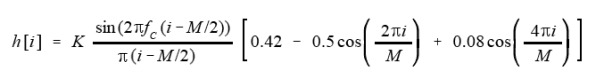
A polyphase filter is a set of subfilters where the filter kernel has been split up into a matrix with each row representing a subfilter.  The input samples are passed into each subfilter that are then summed together to produce the output.  For example, given the impulse response of the filter

we can separate it into two subfilters, E₀ and E₁

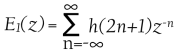
where E₀ contains the even-numbered kernel coefficients and E₁ contains the odd ones.  We can then express H(z) as

This can of course be extended for any number of subfilters.  In fact, the number of subfilters in the polyphase interpolating/decimating filters is exactly the same as the resampling factor.  So if we’re upsampling-downsampling by a factor of 4X, we use 4 subfilters.  However, we still have the problem of filtering on 4 times the number of samples as a result of the upsampling.  Here is where the Noble Identity comes in.  It states that for multirate signal processing, filtering before upsampling and filtering after downsampling is equivalent to filtering after upsampling and before downsampling.

Noble Identities for upsampling and downsampling.

When you think about it, it makes sense.  Recall that upsampling involves zero-insertion between the existing samples.  These 0 values, when passed through the filter, simply evaluate out to 0 and have no effect on the resulting signal, so they are wasted calculations.  We are now able to save a lot of computational expense by filtering prior to upsampling the signal, and then filtering after downsampling.  In other words, the actual filtering takes place at the original sample rate.  The way this works in with the polyphase filter is quite clever: through a commutator switch.

Let’s take the case of decimation first because it’s the easier one to understand.  Before the signal’s samples enter the polyphase filter, a commutator selects every Mth sample (M is the decimation factor) to pass into the filter while discarding the rest.  The results of each subfilter is summed together to produce the signal, back to its original sample rate and without aliasing components.  This is illustrated in the following diagram:

Polyphase decimator with a commutator switch that selects the input.

Interpolation works much the same, but obviously on the other end of the filter.  Each input sample from the signal passes through the polyphase filter, but instead of summing together the subfilers, a commutator switch selects the outputs of the subfilters that make up the resulting upsampled signal.  Think of it this way: one sample passes into each of the subfilters that then results in L outputs (L being the interpolation factor and the number of subfilters).  The following diagram shows this:

Polyphase interpolating filter with a commutator switch that selects the output.

We now have a much more efficient resampling filter.  There are other methods that exist as well to implement a resampling filter, including Fast Fourier Transform, which is a fast and efficient way of doing convolution, and would be a preferred method of implementing FIR filters.  At lower orders however, straight convolution is just as fast (if not even slightly faster at orders less than 60 or so) than FFT; the huge gain in efficiency really only occurs with a kernel length greater than 80 – 100 or so.

Before concluding, let’s look at some C++ code fragments that implement these two polyphase structures.  Previously I had done all the work inside a single method that contained all the for loops to implement the convolution.  Since we’re dealing with a polyphase structure, it naturally follows that the code should be refactored into smaller chunks since each filter branch can be throught of as an individual filter.

First, given the prototype filter’s kernel, we break it up into the subfilter branches.  The number of subfilters (branches) we need is simply equal to the resampling factor.  Each filter branch will then have a length equal to the prototype filter’s kernel length divided by the factor, then +1 to take care of rounding error.  i.e.

branch order = (prototype filter kernel length / factor) + 1

The total order of the polyphase structure will then be equal to the branch order x number of branches, which will be larger than the prototype kernel, but any extra elements should be initialized to 0 so they won’t affect the outcome.

The delay line, z, for the interpolator will have a length equal to the branch order.  Again, each branch can be thought of as a separate filter.  First, here is the decimating resampling code:

 

Example of decimating resampler code.

As can be seen, calculating each polyphase branch is handled by a separate object with its own method of calculating the subfilter (processDownsample).  We index the input signal with variable M, advances at the rate of the resampling factor.  The gain adjust can be more or less ignored depending on how the resampling is implemented.  In my case, I have precalculated the prototype filter kernels to greatly improve efficiency.  However, the interpolation process decreases the level of the signal by an amount equal to the resampling factor in decibels.  In other words, if our factor is 3X, we need to amplify the interpolated signal by 3dB.  I’ve done this by amplifying the prototype filter kernel so I don’t need to adjust the gain during interpolation.  But this means I need to compensate for that in decimation by reducing the level of the signal by the same amount.

Here is the interpolator code:

Example of interpolation resampler code.

As we can see, it’s quite similar to the decimation code, except that the output selector requires an additional for loop to distribute the results of the polyphase branches.  Similarly though, it uses the same polyphase filter object to calculate each filter branch, using the delay line as input instead of the input signal directly.  Here is the code for the polyphase branches:

Code implementing the polyphase branches.

Again, quite similar, but with a few important differences.  The decimation/downsampling MACs the input sample by each kernel value whereas interpolation/upsampling MACs the delay line with the branch kernel.

Hopefully this clears up a bit of confusion regarding the implementation of the polyphase filter.  Though this method splits up and divides the tasks of calculating the resampling into various smaller objects than before, it is much easier to understand and maintain.

Resampling, as we have seen, is not a cheap operation, especially if a strong filter is required.  However, noticeable aliasing will render any audio unusable, and once it’s in the signal it cannot be removed.  Probably the best way to avoid aliasing is to prevent it in the first place by using band-limited oscillators or other methods to keep all frequencies below the Nyquist limit, but this isn’t always possible as I pointed out in Part 1 with ring modulation, distortion effects, etc.  There is really no shortage of challenges to deal with in digital audio!

Audio Resampling: Part 1

Resampling in digital audio has two main uses.  One is to convert audio into a sampling rate needed by a particular system or engine (e.g. converting 48kHz audio to the required 44.1kHz required by CDs).  The second is to avoid aliasing during signal processing by raising the Nyquist limit.  I will be discussing the latter.

Lately I’ve been very busy working on improving and enhancing the sound of ring modulation for a fairly basic plug-in being developed by AlgoRhythm Audio (coming soon).  I say basic becuase as far as ring modulation goes, there are few DSP effects that are simpler in theory and in execution.  Simply take some input signal, multiply it by a carrier signal (usually some kind of oscillator like a sine wave), and we have ring modulation.  The problem that arises, however, and how this connects in with resampling, is that this creates new frequencies in the resulting output that were not present in either signal prior to processing.  These new frequencies created could very well violate the Nyquist limit of the current sampling rate during processing, and that leads us to resampling as a way to clamp down on aliasing frequencies that can be introduced as a result.

Aliasing is an interesting phenomenon that occurs in digital audio, and in every sense of the word is an undesired noise that we need to make sure does not pollute our audio.  There are many resources around that go into more detail on aliasing, but I will give a brief overview of it with some audio and visual samples.

Aliasing occurs when there are frequencies present in a signal that are greater than the Nyquist limit (half of the sampling rate).  What happens in such a case is that the sampling rate is not high enough to properly capture (sample) the high frequency of the signal, and so the frequency “folds over” and creates aliases that are mirror images of the original frequency.  Here, for example, is a square wave at 4000Hz created using 20 harmonics at a sampling rate of 44.1kHz (keep in mind that 4000Hz is the fundamental frequency, and that square waves contain many additional frequencies above that depending on how many harmonics were used to create it, so in this case Nyquist is still being violated):

4000Hz square wave with aliasing

Notice the low tone below the actual 4000Hz frequency.  Here is the resulting waveform of this square wave that shows us visually that we’re not sampling fast enough to accurately reproduce the waveform.  Notice the inconsistencies in the waveform.

Now, going to the extreme a bit, here is the same square wave sampled at a rate of 192kHz.

4000Hz square wave with no aliasing

It’s a pure 4000Hz square wave tone.  Examining the waveform of this square wave shows us that the sampling rate was more that adequate to reproduce this signal digitally:

Not all signal processing effects are susceptible to aliasing, and certainly not to the same degree.  Because ring modulation produces additional inharmonic frequencies, it is a prime example of a process that is easily affected by aliasing.  Others include distortion and various other kinds of modulation techniques (especially when taken to the extreme).  However, ring modulation with a sine wave is generally safe as long as the frequency of the sine wave is kept  low enough because sine waves have no harmonics to them, only the fundamental.  Introducing other wavetypes into this process, however, can quite easily bring about aliasing.

Here is an example of ring modulation with a sawtooth wave sweeping up from about 200Hz to 5000Hz.  As it glides up, you will be able to hear the aliasing kicking in at around 0:16 or so.  The example with no aliasing has been upsampled by 3X before processing, then downsampled by 3X back to its original rate.

Ring modulation with a sawtooth sweep, with aliasing

Ring modulation with sawtooth sweep, with no aliasing

So how does upsampling and downsampling work?  In theory, and even to some extent in practice, it’s very straightforward.  The issue, as we will see, is in making it efficient and fast.  In DSP we’re always concerning ourselves with speedy execution times to avoid latency or audio dropouts or running out of memory, etc.

To upsample, we insert 0-valued samples in between every L-th (our upsampling factor) original sample.  (i.e. upsampling by 3X, [1, 2, 3, 4] becomes [1,0,0,2,0,0,3,0,0…])  However, this introduces aliasing into our audio so we need to interpolate these values so that they “join” the sample values of the original waveform.  This is accomplished by using an interpolating low-pass filter.  This entire process is known as interpolation.

Dowsampling is much the same.  We remove every M-th (our downsampling factor) sample from the original signal.  (i.e. downsampling by 2X, [1,2,3,4,5] becomes [1,3,5…])  This process does not introduce aliasing, but we do need to make sure the Nyquist limit is adhered to at the new sampling rate by low-pass filtering with a cutoff frequency at the new Nyquist rate.  This entire process is known as decimation.

Fairly straightforward.  Proceeding with this method, however, would be known as brute force — generally not a good way to go.  The reason why becomes clearer when we consider what kind of low-pass filter we need for this operation.  The ideal filter would be one that would brick-wall attenuate all frequencies higher than Nyquist and leave everything else untouched (thus preserving all the frequencies and tonal content of our original audio).  This is, alas, impossible, as it would require an infinitely long filter kernel.  The function that would implement this ideal filter is the rectangular function.

The rectangular function.

By taking the Fourier transform of the rectangular function we end up with the sinc function, which is given by:

y(x) = sin (x) / x, which becomes y(x) = sin (πx) / πx for signal processing.

Graph of the sinc function, sin (πx) / πx

The sinc functions trails on for infinity in both directions, which can be seen in the graph above, so we need to enforce bounds around it by applying a window function.  Windowing is a method of designing FIR filters by essentially “surrounding” a function (in our case the sinc) by the window, which enforces bounds so that we can properly derive a filter kernel for use in calculations.  The rectangular function shown above is a type of window, but as I mentioned, infinite slope is a deal-breaker in audio.

The Blackman window, given by the function

w(i) = 0.42 – 0.5 cos(2πi / M) + 0.08 cos(4πi / M),

where M is the length of the filter kernel, is a good choice for resampling because it offers a good stop-band attenuation of -74dB with good rolloff.  Putting this together with the sinc function, we can derive the filter kernel with the following formula:

Windowed-sinc kernel formula*

where f_c is the normalized cutoff frequency.  When i = M/2, to avoid a divide by zero, h(i) = 2f_c.  K is a constant value used to achieve unity gain at zero frequency and can be ignored while calculating the kernel coefficients.  After all coefficients have been calculated, K can be found by summing together all the coefficients, h(i), and then dividing each by the resulting sum.

* Source: Smith, Steven W., “The Scientist and Engineer’s Guide to Digital Signal Processing”, Chapter 16.

Now that we have the filter design, let’s consider the properties of the FIR filter and compare them to IIR filter designs.  IIR filters give us better performance and attenuation at lower orders, meaning that they execute faster and perform better with fewer calculations than FIR filters.  However, IIR filters are still not powerful enough, even at slightly higher orders, to give us the performance we need for resampling, and trying to push IIR filters into very high orders can make them unstable and/or susceptible to quantization error due to the nature of recursion.  IIR filters also do not offer linear phase response.  FIR filters are the better choice for these reasons, but the unfortunate drawback is that they execute slowly due to being implemented by convolution.  In addition, they need to be pushed to high orders to give us the performance needed for attenuating aliasing frequencies.

However, the order of the interpolating low-pass filter can be negotiated based on the frequency content of the audio signal(s) involved.  If the audio is sufficiently oversampled, it will not contain enough frequencies near Nyquist, and as such a lower order filter can be used with a gentler rolloff without adversely affecting the audio and attenuating actual frequencies in the signal.  There are plenty of cases where we just don’t know the frequency content of the audio signals involved in processing, however, so a strong filter may be needed in these cases.  Here is a graph of a 264-order window-sinc filter (in other words, a filter kernel of length 265 including the sample x(0)):

264-order window-sinc low-pass filter frequency response (cutoff frequency at 10kHz, resulting in a transition band of 882Hz)

With this in consideration, it can be easy to see that convolving a signal with a 264-order FIR filter is computationally costly for real-time processing.  There are a number of ways to improve upon this when it comes to resampling.  One is using the FFT to apply the filter.  Another interesting solution is to combine the upsampling/downsampling process into the filter itself, which can further be optimized by turning it into a polyphase filter.

The theory and implementation of a polyphase filter is a fairly long and involved topic on its own so that will be forthcoming in part 2,where we look at how to implement resampling efficiently.