Dynamics Processing: Compressor/Limiter, part 3

In part 1 of this series of posts, I went over creating an envelope detector that detects both peak amplitude and RMS values. In part 2, I used it to create a compressor/limiter. There were two common features missing from that compressor plug-in, however, that I will go over in this final part: soft knee and lookahead. Also, as I have stated in the previous parts, this effect is being created with Unity in mind, but the theory and code is easily adaptable to other uses.

Let’s start with lookahead since it is very straightforward to implement. Lookahead is common in limiters and compressors because any non-zero attack/release times will cause the envelope to lag behind the audio due to the filtering, and as a result, it won’t attenuate the right part of the signal corresponding to the envelope. This can be fixed by delaying the output of the audio so that it lines up with the signal’s envelope. The amount we delay the audio by is the lookahead time, so an extra field is needed in the compressor:

public class Compressor : MonoBehaviour
{
    [AudioSlider("Threshold (dB)", -60f, 0f)]
    public float threshold = 0f;		// in dB
    [AudioSlider("Ratio (x:1)", 1f, 20f)]
    public float ratio = 1f;
    [AudioSlider("Knee", 0f, 1f)]
    public float knee = 0.2f;
    [AudioSlider("Pre-gain (dB)", -12f, 24f)]
    public float preGain = 0f;			// in dB, amplifies the audio signal prior to envelope detection.
    [AudioSlider("Post-gain (dB)", -12f, 24f)]
    public float postGain = 0f;			// in dB, amplifies the audio signal after compression.
    [AudioSlider("Attack time (ms)", 0f, 200f)]
    public float attackTime = 10f;		// in ms
    [AudioSlider("Release time (ms)", 10f, 3000f)]
    public float releaseTime = 50f;		// in ms
    [AudioSlider("Lookahead time (ms)", 0, 200f)]
    public float lookaheadTime = 0f;	// in ms

    public ProcessType processType = ProcessType.Compressor;
    public DetectionMode detectMode = DetectionMode.Peak;

    private EnvelopeDetector[] m_EnvelopeDetector;
    private Delay m_LookaheadDelay;

    private delegate float SlopeCalculation (float ratio);
    private SlopeCalculation m_SlopeFunc;

    // Continued...

I won’t actually go over implementing the delay itself since it is very straightforward (it’s just a simple circular buffer delay line). The one thing I will say is that if you want the lookahead time to be modifiable in real time, the circular buffer needs to be initialized to a maximum length allowed by the lookahead time (in my case 200ms), and then you need to keep track of the actual time/position in the buffer that will move based on the current delay time.

The delay comes after the envelope is extracted from the audio signal and before the compressor gain is applied:

void OnAudioFilterRead (float[] data, int numChannels)
{
    // Calculate pre-gain & extract envelope
    // ...

    // Delay the incoming signal for lookahead.
    if (lookaheadTime > 0f) {
        m_LookaheadDelay.SetDelayTime(lookaheadTime, sampleRate);
        m_LookaheadDelay.Process(data, numChannels);
    }

    // Apply compressor gain
    // ...
}

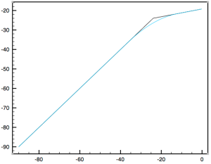
That’s all there is to the lookahead, so now we turn our attention to the last feature. The knee of the compressor is the area around the threshold where compression kicks in. This can either be a hard knee (the compressor kicks in abruptly as soon as the threshold is reached) or a soft knee (compression is more gradual around the threshold, known as the knee width). Comparing the two in a plot illustrates the difference clearly.

Hard knee in black and soft knee in light blue (threshold is -24 dB).

There are two common ways of specifying the knee width. One is an absolute value in dB, and the other is as a factor of the threshold as a value between 0 and 1. The latter is one that I’ve found to be most common, so it will be what I use. In the diagram above, for example, the threshold is -24 dB, so a knee value of 1.0 results in a knee width of 24 dB around the threshold. Like the lookahead feature, a new field will be required:

public class Compressor : MonoBehaviour
{
    [AudioSlider("Threshold (dB)", -60f, 0f)]
    public float threshold = 0f;		// in dB
    [AudioSlider("Ratio (x:1)", 1f, 20f)]
    public float ratio = 1f;
    [AudioSlider("Knee", 0f, 1f)]
    public float knee = 0.2f;
    [AudioSlider("Pre-gain (dB)", -12f, 24f)]
    public float preGain = 0f;			// in dB, amplifies the audio signal prior to envelope detection.
    [AudioSlider("Post-gain (dB)", -12f, 24f)]
    public float postGain = 0f;			// in dB, amplifies the audio signal after compression.
    [AudioSlider("Attack time (ms)", 0f, 200f)]
    public float attackTime = 10f;		// in ms
    [AudioSlider("Release time (ms)", 10f, 3000f)]
    public float releaseTime = 50f;		// in ms
    [AudioSlider("Lookahead time (ms)", 0, 200f)]
    public float lookaheadTime = 0f;	// in ms

    public ProcessType processType = ProcessType.Compressor;
    public DetectionMode detectMode = DetectionMode.Peak;

    private EnvelopeDetector[] m_EnvelopeDetector;
    private Delay m_LookaheadDelay;

    private delegate float SlopeCalculation (float ratio);
    private SlopeCalculation m_SlopeFunc;

    // Continued...

At the start of our process block (OnAudioFilterRead()), we set up for a possible soft knee compression:

float kneeWidth = threshold * knee * -1f; // Threshold is in dB and will always be either 0 or negative, so * by -1 to make positive.
float lowerKneeBound = threshold - (kneeWidth / 2f);
float upperKneeBound = threshold + (kneeWidth / 2f);

Still in the processing block, we calculate the compressor slope as normal according to the equation from part 2:

slope = 1 – (1 / ratio), for compression

slope = 1, for limiting

To calculate the actual soft knee, I will use linear interpolation. First I check if the knee width is > 0 for a soft knee. If it is, the slope value is scaled by the linear interpolation factor if the envelope value is within the knee bounds:

slope *= ((envValue – lowerKneeBound) / kneeWidth) * 0.5

The compressor gain is then determined using the same equation as before, except instead of calculating in relation to the threshold, we use the lower knee bound:

gain = slope * (lowerKneeBound – envValue)

The rest of the calculation is the same:

for (int i = 0, j = 0; i < data.Length; i+=numChannels, ++j) {
    envValue = AudioUtil.Amp2dB(envelopeData[0][j]);
    slope = m_SlopeFunc(ratio);

    if (kneeWidth > 0f && envValue > lowerKneeBound && envValue < upperKneeBound) { // Soft knee
        // Lerp the compressor slope value.
        // Slope is multiplied by 0.5 since the gain is calculated in relation to the lower knee bound for soft knee.
        // Otherwise, the interpolation's peak will be reached at the threshold instead of at the upper knee bound.
        slope *= ( ((envValue - lowerKneeBound) / kneeWidth) * 0.5f );
        gain = slope * (lowerKneeBound - envValue);
    } else { // Hard knee
        gain = slope * (threshold - envValue);
        gain = Mathf.Min(0f, gain);
    }

    gain = AudioUtil.dB2Amp(gain);

    for (int chan = 0; chan < numChannels; ++chan) {
        data[i+chan] *= (gain * postGainAmp);
    }
}

In order to verify that the soft knee is calculated correctly, it is best to plot the results. To do this I just created a helper method that calculates the compressor values for a range of input values from -90 dB to 0 dB. Here is the plot of a compressor with a threshold of -12.5 dB, a 4:1 ratio, and a knee of 0.4:

Compressor with a threshold of -12.5 dB, 4:1 ratio, and knee of 0.4.

Of course this also works when the compressor is in limiter mode, which will result in a gentler application of the limiting effect.

Compressor in limiter mode with a threshold of -18 dB, and knee of 0.6.

That concludes this series on building a compressor/limiter component.

AdVerb: Building a Reverb Plug-In Using Modulating Comb Filters

Some time ago, I began exploring the early reverb algorithms of Schroeder and Moorer, whose work dates back all the way to the 1960s and 70s respectively.  Still their designs and theories inform the making of algorithmic reverbs today.  Recently I took it upon myself to continue experimenting with the Moorer design I left off with in an earlier post.  This resulted in the complete reverb plug-in “AdVerb”, which is available for free in downloads.  Let me share what went into designing and implementing this effect.

One of the foremost challenges in basing a reverb design on Schroeder or Moorer is that it tends to sound a little metallic because with the number of comb filters suggested, the echo density doesn’t build up fast or dense enough.  The all-pass filters in series that come after the comb filter section helps to diffuse the reverb tail, but I found that the delaying all-pass filters added a little metallic sound of their own.  One obvious way of overcoming this is to add more comb filters (today’s computers can certainly handle it).  More importantly, however, the delay times of the comb filters need to be mutually prime so that their frequency responses don’t overlap, which would result in increased beating in the reverb tail.

To arrive at my values for the 8 comb filters I’m using, I wrote a simple little script that calculated the greatest common divisor between all the delay times I chose and made sure that the results were 1.  This required a little bit of tweaking in the numbers, as you can imagine finding 8 coprimes is not as easy as it sounds, especially when trying to keep the range minimal between them.  It’s not as important for the two all-pass filters to be mutually prime because they are in series, not in parallel like the comb filters.

I also discovered, after a number of tests, that the tap delay used to generate the early reflections (based on Moorer’s design) was causing some problems in my sound.  I’m still a bit unsure as to why, though it could be poorly chosen tap delay times or something to do with mixing, but it was enough so that I decided to discard the tap delay network and just focus on comb filters and all-pass filters.  It was then that I took an idea from Dattorro and Frenette who both showed how the use of modulated comb/all-pass filters can help smear the echo density and add warmth to the reverb.  Dattorro is responsible for the well-known plate reverbs that use modulating all-pass filters in series.

The idea behind a modulated delay line is that some oscillator (usually a low-frequency sine wave) modulates the delay value according to a frequency rate and amplitude.  This is actually the basis for chorusing and flanging effects.  In a reverb, however, the values need to be kept very small so that the chorusing effect will not be evident.

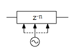
I had fun experimenting with these modulated delay lines, and so I eventually decided to modulate one of the all-pass filters as well and give control of it to the user, which offers a great deal more fun and crazy ways to use this plug-in.  Let’s take a look at the modulated all-pass filter (the modulated comb filter is very similar).  We already know what an all-pass filter looks like, so here’s just the modulated delay line:

Modulated all-pass filter.

The oscillator modulates the value currently in the delay line that we then use to interpolate, resulting in the actual value.  In code it looks like this:

double offset, read_offset, fraction, next;
size_t read_pos;

offset = (delay_length / 2.) * (1. + sin(phase) * depth);
phase += phase_incr;
if (phase > TWO_PI) phase -= TWO_PI;
if (offset > delay_length) offset = delay_length;

read_offset = ((size_t)delay_buffer->p - (size_t)delay_buffer->p_head) / sizeof(double) - offset;
if (read_offset  delay_length) {
    read_offset = read_offset - delay_length;
}

read_pos = (size_t)read_offset;
fraction = read_offset - read_pos;
if (read_pos != delay_length - 1) {
    next = *(delay_buffer->p_head + read_pos + 1);
} else {
    next = *delay_buffer->p_head;
}

return *(delay_buffer->p_head + read_pos) + fraction * (next - *(delay_buffer->p_head + read_pos));

In case that looks a little daunting, we’ll step through the C code (apologies for the pointer arithmetic!).  At the top we calculate the offset using the delay length in samples as our base point.  The following lines are easily seen as incrementing and wrapping the phase of the oscillator as well as capping the offset to the delay length.

The next line calculates the current position in the buffer from the current position pointer, p, and the buffer head, p_head.  This is accomplished by casting the pointer addresses to integral values and dividing by the size of the data type of each buffer element.  The read_offset position will determine where in the delay buffer we read from, so it needs to be clamped to the buffer’s length as well.

The rest is simply linear interpolation (albeit with some pointer arithmetic: delay_buffer->p_head + read_pos + 1 is equivalent to delay_buffer[read_pos + 1]).  Once we have our modulated delay value, we can finish processing the all-pass filter:

delay_val = get_modulated_delay_value(allpass_filter);

// don't write the modulated delay_val into the buffer, only use it for the output sample
*delay_buffer->p = sample_in + (*delay_buffer->p * allpass_filter->g);
sample_out = delay_val - (allpass_filter->g * sample_in);

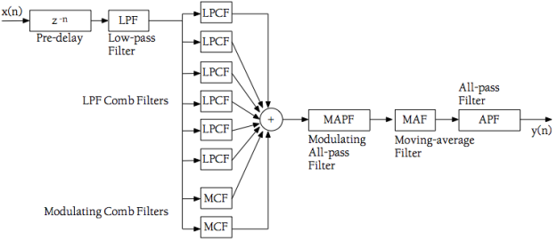
The final topology of the reverb is given below:

Topology of the AdVerb plug-in.

The pre-delay is implemented by a simple delay line, and the low-pass filters are of the one-pole IIR variety.  Putting the LPFs inside the comb filters’ feedback loops simulates the absorption of energy that sound undergoes as it comes in contact with surfaces and travels through air.  This factor can be controlled with a damping parameter in the plug-in.

The one-pole moving-average filter is there for an extra bit of high frequency roll-off, and I chose it because this particular filter is an FIR type and has linear phase so it won’t add further disturbance to the modulated samples entering it.  The last (normal) all-pass filter in the series serves to add extra diffusion to the reverb tail.

Here are some short sound samples using a selection of presets included in the plug-in:

Piano, “Medium Room” preset

The preceding sample demonstrates a normal reverb setting.  Following are a few samples that demonstrate a couple of subtle and not-so-subtle effects:

Piano, “Make it Vintage” preset

Piano, “Bad Grammar” preset

Flute, “Shimmering Tail” preset

Feel free to get in touch regarding any questions or comments on “AdVerb“.

The Making of a Plug-In: Part 1

Well, it’s finally time to do something useful with all this stuff.  Not that command-line programs aren’t useful, but they have their limitations — especially these days.  Making a plug-in is a great way to apply all the things I’ve been doing, which really culminates into making a deliverable product that has a use.  I have thus decided to make a Match Envelope plug-in, inspired by a suggestion from my good friend Igor (thanks man!).  This first part of the “making of” blog will cover some of the initial conception and development of the prototype program as well as introducing some of the planned features and parameters of the plug-in.  Focus will not be on actual C++ code at this point, but more on the math and the concepts behind it.

This Match Envelope plug-in will be similar in many ways to an Envelope Follower.  It extracts the envelope from a source audio file and applies it to a destination audio file.  Envelope followers tend to be more geared towards MIDI and there are not too many (to my knowledge) stand-alone plug-ins that give you what you need.  They can also be found as features in filters and other kinds of plug-ins.

The usefulness of them can vary quite a bit as we will see in more detail.  Commonly we see Envelope Followers used to sync up a sound to a drum loop for example.  Another benefit of using this plug-in involves layering sounds together.  If a seamless blend is desired, the envelopes of the different layers must match fairly close or else we will hear the distinct layers.  With a mix of more percussive sounds with sustained ones, an envelope matcher can be quite useful.

Furthermore, Match Envelope can be used to approximate the attack or release of instruments in an orchestra that have been recorded.  Let’s say you wish to double the flute line, or even the bass line with something; the Match Envelope plug-in can assist in blending the two layers together.  As will be discussed below, there will be parameters and features to control the effect because there are situations where we certainly don’t want a “lifeless” 100% match.

In addition to its uses in music, it can also be used in sound design, where layers upon layers of different sound sources are often combined to great effect.  Given some of the cool and varied applications of this plug-in, and considering that there are not a great many of them out there, I felt this was an exciting project to take on!

So how does it work and where do we start?  To extract the envelope shape from the source audio, we use windows of a certain size that will either take the peak amplitude or the average amplitude within that window and store it in a buffer.  We then take those amplitude values and apply them onto the destination audio, effectively recreating its amplitude shape.  Fairly straightforward in concept, but there’s more to it than that.

If we just apply the extracted envelope values to the audio, we’ll get a staircase.  Thus we turn to interpolation.  At first I went with linear interpolation, given by the formula

where we want y(x) with position x between points (x₀, y₀) and (x₁, y₁), and this resulted in a fairly good and accurate match.  However, we need a better quality interpolation; one that will give us a smoother, more accurate curve that will result in better quality audio.  For this we turn to cubic interpolation.  The cubic equation will look familiar to most;

but as it has four unknowns (the coefficients a, b, c, d) we need four points in order to interpolate or solve it (remember that from math class?).  Solving this equation isn’t terribly complicated; we take the derivative of y(x) and then solve both equations for x = 0 and x = 1.  This assumes that the distance between successive x values is 1.  For a more detailed explanation of how to solve this equation for the coefficients go here: http://www.paulinternet.nl/?page=bicubic

There was one problem I encountered after implementing this, however, that is worth mentioning.  My window sizes were not of the unit value (1) and even moreso, can be changed by the user, so I did not have a constant for the distance between x values.  The solution is pretty simple (almost too much so as I was heavily focused on workarounds that were far too complex).  Basically we just scale the x increment value, which keeps track of our position, by the inverse of the window duration.

Let’s say we set our window duration to 20 milliseconds.  That gives us our window size of 882 samples (assuming a sample rate of 44.1kHz).  Our x increment value is then 2.268×10^-5 (0.02 / 882) based on a window size of 0.02.  But we need a window size that is effectively 1, so 1 / 0.02 is 50, and this is our scaling factor.  The increment value is now 1.1334×10^-3.

One final detail that caused a small issue was rounding error.  At the boundaries of some windows, I would end up with an x value of 3.999999 or similar.  This caused sample error that did not sound very good, but the solution was a simple matter of adding a very small value to the x position at the end of each window loop (0.0000001 for instance).  Some additional testing with varying window sizes will be done to make sure no more sample/rounding error occurs.

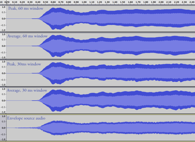
While on the topic of windows, their function is to affect the smoothness of the extracted envelope as well as its accuracy.  Smaller window sizes will result in a closer match to the source audio’s envelope, and larger ones will be more of an approximation.  Before moving on, let’s get a visual of how I’m testing out the functionality of the plug-in.

To really get a good idea of how the program is working, using something simple like a triangle wave is great for visualizing the outcome.

As I mentioned previously, there are two ways of taking the amplitude within each window: taking the maximum (peak) value, or taking the average.  Just below we see the difference between them, and it is the intention at this point to have this as an option for which to use.

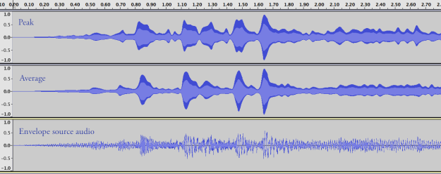
Here we can see a number of things already at work.  The difference between peak and average amplitude is not very much.  But in this case, the source audio is quite smooth and the destination waveform is completely constant.  A following example will demonstrate the difference between these better.  We also see the effects of different window sizes in the visual above.  A very large window size (perhaps around 500 ms to 1 s) would retain much more of the shape of the destination audio and might be more useful for longer sustained sounds, while a shorter window length is better for capturing percussive sounds.  The example below uses a different audio as the source, with more percussive attacks.

There is a clear difference between peak and average, at least visually.  We will hear at the end of this post that they don’t differ a huge amount to our ears (at least not with these examples).

Before I wrap up this post, I want to discuss two additional features I’m planning at this point.  One is just a simple gain, that scales the result of the envelope match.  An extension of this feature will be to add an option where the user can specify that the amplitude at the end of the envelope will match the amplitude of the rest of the audio (i.e. at the junction point where the envelope ends, and the rest of the audio continues unmodified).  This would be useful if the user just wants to match a section from a source audio file.

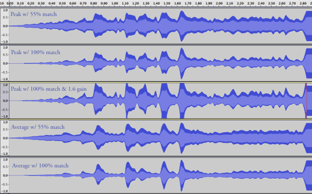
Secondly, I have implemented a parameter called “match strength %” that will control how strongly the envelope will modify the destination audio.  The cool thing about this is that it’s proportional to the difference in amplitude between the envelope and the destination audio.  To accomplish this, I scale the interpolated value, ival, by the equation

where buffer is the amplitude of the destination audio and a is a value in % specified by the user.  We can see it visually in the image below.

The bigger the distance between the two amplitudes, the stronger the envelope affects the audio.  This ensures that the general shape of the envelope remains, while retaining more of the original shape in relation to the specified % by the user.  The middle waveform shows a gain factor of 1.6, but this was incorrectly implemented, as the gain modifies the interpolated value, ival, instead of the result of ival * buffer.  As it is in the image above, gain is also proportional, but I intend it to be a linear effect.

Here are a couple of examples of how this process sounds at this stage.  These audio samples use just the triangle wave that I have been using to test the program layered on top of the audio I extracted the envelope from.  Listen to how the triangle wave follows the shape of the audio and see if you can hear a difference between the peak version and the average version (the peak version has slightly stronger attacks from the triangle wave).

Peak windowing: layered triangle wave over source audio

Average windowing: layered triangle wave over source audio

This has been a long and wordy post, so it’s time to wrap up.  I’m pleased so far with the functionality and behavior of the plug-in and the parameters and features I am planning on implementing.  It should provide a good amount of flexibility to shape a given waveform/audio file from an extracted envelope source, and should have some fun and productive uses.